This blogpost will teach you set up automated email reports to view how search volumes i.e. Google Trends vary over time.

The email report will also include important search terms that are “rising” or near a “breakout point”. This can be really useful as the breakout keywords indicate users across the globe have recently started paying great attention to these search terms. So you could create original content to attract people using these phrases in their Google searches. This is an amazing way to boost traffic/ sales leads, etc. by taking advantage of new trends.
Note, that the results are relative, not absolute search volume terms. But it is still quite useful, as you could narrow down your keywords list, and login to Adsense/ keyword planner to get the exact search volume. Export the list from this script to a .csv and simply upload in Adsense. It also gives you a clear indication of how search volumes compare across similar terms – classic SEO !
We will perform all our data pull requests and manipulations in R. The best part is that you do not need any API keys or logins for this tutorial!
[ Do you know what else is trending? My book on how to get hired as a datascientist. Check it out on Amazon, where it is the #1 NEW RELEASE and top 10 in its categories. Whether you are currently enrolled in a data science course or actively job searching, this book is sure to help you attract multiple job offers in this lucrative niche. ]
Without further interruptions – let’s dive right in to the trend analysis.
Step 1 – Load Libraries
Start by loading the libraries – “gtrends” is the main library package which will help us pull data for search results.
library (gtrendsR)
library(ggplot2)
library(plotly)
library(dplyr)
library(sqldf)
library(reshape2)
Step 2 – Search terms and timeframe
We need to specify the variables we need to pass to the search query:
- search terms of interest. Unfortunately, you can only pass 5 terms at one time. Theoretically you could store the value and repeat the searches, but since numbers are relative, make sure that you keep at least one term in common and then normalize.
- Remember, we get relative search volumes (max = 100); NOT absolute volumes!
- timeframe under consideration, has to be in the format “YYYY-mm-dd” ONLY. No exceptions. End date = today, whereas start date will be the the first of the month, six months ago.
- country codes – I’ve only used “US”, but you can search for multiple countries using a string array like c(“US”, “CA”, “DE”) which stands for US, Canada and Germany.
- Channels – default is “web”, but you can search for “new” or “images”. Images would be good for those promoting content in Pinterest or Instagram.
date6mthpast <- Sys.Date() – 180
startdate <- paste0( substr(as.character(date6mthpast), 1,7), “-01”, sep = “”)
currdate = as.character(Sys.Date())
timeframe = paste( startdate, currdate)
keywords <- c(“Data Science jobs”, “MS Analytics Jobs”, “Analytics jobs”,
“Data Scientist course”, “job search”)
country=c(‘US’)
channel=’web’
We will use the gtrends() function to pull the data. This function returns a list of variables and dataframes. Of main interest to us is the “interest_over_time” data frame, “interest_by_region” (state names mostly). There is also a dataframe named “interest_by_city”. The first one does hold data with date value, while the others do not, so it will be aggregated over the entire data frame. I worked around this by pulling once for 6 months, and again for the last 45 days.
trends = gtrends(keywords, gprop =channel,geo=country, time = timeframe )
Step 3 – Search Volume over time
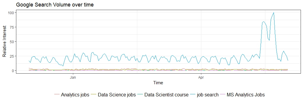
We will use the ggplot function to get a graphical representation of the search volume.
ggplot(data=time_trend, aes(x=date, y=hitval, group=keyword, col=keyword))+
geom_line()+xlab(‘Time’)+ylab(‘Relative Interest’)+ theme_bw() +
theme(legend.title = element_blank(), legend.position=”bottom”, legend.text=element_text(size=12)) +
ggtitle(“Google Search Volume over time”)

Notice that the interest in term “job search” is significantly higher than any other keyword and spike in April and May (people graduating maybe?) This makes sense as it is a more generic term, and applies to larger number of users. On a similar vein, look at the volumes for “MS analytics jobs” . It is almost nil, so clearly a non-starter in terms of targeting.
Step 4 – Interest by Regions
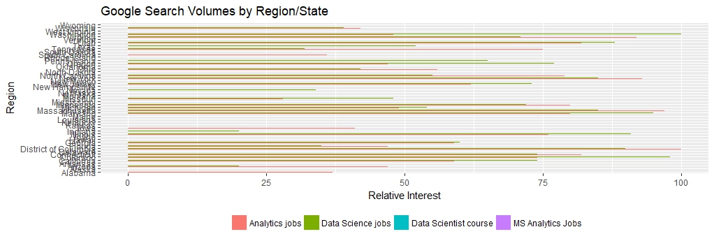
Let us look at interest by region (state names in the US ) . This might be useful to target folks by region, or even location-based ads.
locsearch = trends$interest_by_region
plot2 <- ggplot(subset(locsearch, locsearch$keyword != “job search”),
aes(x=as.factor(location), y= hits, fill=as.factor(keyword) )) +
geom_bar(position=”dodge”, stat=”identity”) +
coord_flip() +
theme(legend.title = element_blank(), legend.position=”bottom”, legend.text=element_text(size=9)) +
xlab(‘Region’)+ ylab(‘Relative Interest’) +
ggtitle(“Google Search Volumes by Region/State”)

Note, that “data scientist course” has almost zero interest compared to broader terms like “analytics jobs” or “datascience Jobs”. Interestingly, “analytics jobs” seems to be a preferred term over “data science” only in NY, MA and Washington DC.
Step 5 – Trending Terms
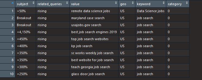
The original list also returns a dataframe titled “related_queries”. Some of these can have tags as “rising” or “breakout”. These are the terms we would like to know as they occur.
breakoutdf = reltopicdf[reltopicdf$related_queries == ‘rising’,]
volbrkdf = breakoutdf[1:10,]
row.names(volbrkdf) = NULL
volbrkdf

Step 6 – Create pdf for email attachments
We will use the pdf() command to create an attachment with all the graphs and add to the email we want to send/receive on a daily basis.
filename2 = paste0(“Google Search Trends – “, Sys.Date(), “.pdf”)
pdf(paste0(“Google Search Trends – “, Sys.Date(), “.pdf”))
plot1
plot2
print(volbrkdf)
dev.off()
dev.off()
If you want to embed one of these figures in the email itself, instead of attachment then please see my post on automated reports.
Step 7 – Send the email
We use the RDCOM library to send out emails. You do need to have Outlook mail client on your PC.
library(RDCOMClient)
OutApp <- COMCreate(“Outlook.Application”)
outMail = OutApp$CreateItem(0)
outMail[[“To”]] = “an**@gmail.com”
outMail[[“subject”]] = paste(“Google Search Trend Report -“, Sys.Date())
email_body1 <- “Write email body content with correct html tags”
outMail[[“HTMLBody”]] = email_body1
file_location = paste0(paste0(abs_path,”/”),filename2)
outMail[[“Attachments”]]$Add(file_location)
outMail
outMail$Send()
The first time you run this, you might need to “allow” RStudio to access your email account. Just add this script to a task scheduler, and choose frequency of delivery, and you are all set! Note, a dummy email address is used, so remember to change the recipient address.
Try it out and let me know if you have any questions, or run into errors. The script is available on the Projects page – link here
Last but not the least, if you are interested in getting hired in a data science field, then please do take at my job-search book. Here is the Amazon link.
Happy Coding!