In this post we are going to analyze stock prices for company Facebook and create a linear regression model.
Code Overview:
Our code performs the following functions. You can download the code here.
- Load original dataset.
- Add data to benchmark against S&P500 data.
- Create derived variables. We create variables to store calculations for the following:
- Date values: split composite dates into day, month and year.
- Daily volatility : Price change between daily high and low prices or intraday change in price. A bigger difference signifies heavy volatility.
- Inter-day price volatility : Price change from previous day
- Data visualization to validate relationship between target variable and predictors.
- Create Linear Regression Model
Step 1&2 – Load Datasets
We load stock prices for Facebook and S&P500. Note, the S&P500 index prices begin from 2004, whereas Facebook was listed as a public company only in May 2012.
We specify “all.x = TRUE” in the merge command to indicate that we do not want dates which are not present in the Facebook file.
fbknew = merge(fbkdf, sp5k, by = “Date”, all.x = TRUE)
Note, we obtained this data from the Yahoo! Finance homepage using the tab “Historical Data”.
Step 3 – Derived Variables
a) Date Values:
The as.Date() function is an excellent choice to breakdown the date variable into day, month and year. The beauty of this function is that it allows you to specify the format of the date in the original data since different regions format it differently. (mmddyyyy / ddmmyy/ ..)
fbknew$Date2 = as.Date(fbknew$Date, “%Y-%m-%d”)
fbknew$mthyr = paste(as.numeric(format(fbknew$Date2, “%m”)), “-“,
as.numeric(format(fbknew$Date2, “%Y”)), sep = “”)
fbknew$mth = as.numeric(format(fbknew$Date2, “%m”))
fbknew$year = as.numeric(format(fbknew$Date2, “%Y”))
b) Intraday price:
fbknew$prc_change = fbknew$High – fbknew$Low
We have only calculated the difference between the High and Low, but since data is available for “Open” and “Close” you can calculate the maximum range as a self-exercise.
Another interesting exercise would be to calculate the average of both, or create a weighted variable to capture the impact of all 4 variables.
c) Inter-day price:
We first sort by date, using the order() function, and then use a “for loop” to calculate price difference from the previous day. Note, since we are working with dataframes we cannot use a simple subtraction command like x = var[i] – var[i-1]. Feel free to try, the error message is really beneficial in understanding how arrays and dataframes differ!
Step 4 – Data Visualization
Before we create any statistical model, it is always good practice to visually explore the relationships between target variable (here “opening price”) and the predictor variables.
With linear regression model, it is more so, to identify if any variables show a non-linear (exponential, parabolic ) relationship. If you see such patterns you can still use linear regression, after you normalize the data using a log function.
Here are some of the charts from such an exploration between “Open” price (OP) and other variables. Note there may be multiple explanations for the relationship, here we are only looking at the patterns, not the reason behind it.
a) OP versus Trade Volume:
From chart below it looks like the volume is inversely related to price. There is also one outlier (last data point) . We use the lines() and lowess() functions to add a smooth trendline.
An interesting self-exercise would be to identify the date when this occurred and match it to a specific event in the company history (perhaps the stock split?)
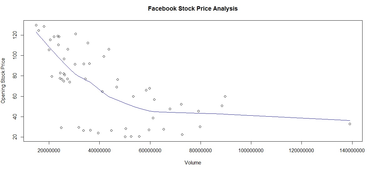
Facebook Stock – Trading Volume versus Opening Stock Price
b) OP by Month & Year:
We see that the stock price has been steadily increasing year on year.
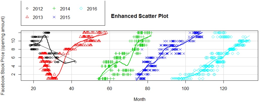
Facebook price by month and year
c) OP versus S&P500 index price:
Clearly the Facecbook stock price has a linear relationship with S&P500 index price (logical too!)
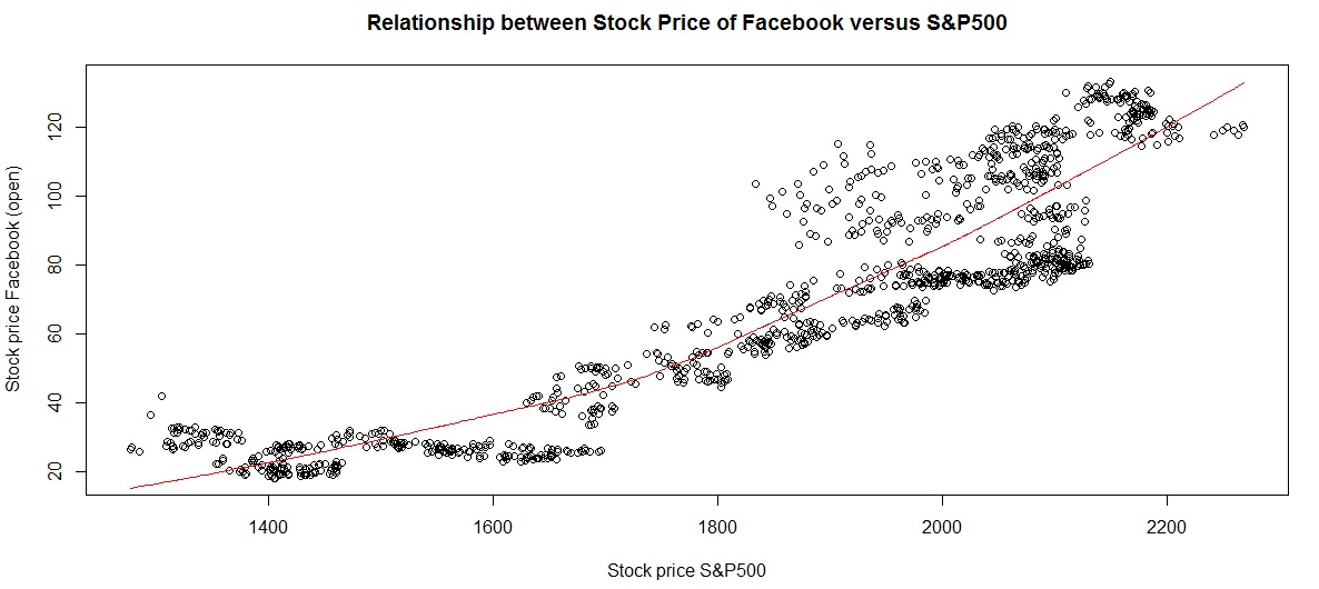
Facebook stock price versus S&P500 performance
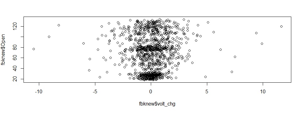
d) Daily volatility:
This is slightly scattered although the central clustering of data points indicates this as a fairly stable.
 Note, we use the sqldf package to aggregate data by monthyear / month for some of these charts.
Step 5 – Linear Regression Model
Our model formula is as follows:
lmodelfb = lm(Open ~ High + Volume + SP500_price + prc_change + mthyr + mth + year + volt_chg, data = fbknew)
summary(lmodelfb)
We use the summary function to view the intercepts and identify the predictors with the biggest impact, as shown in table below:
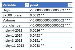
We see that price is affected overall by S&P500, interday volatility and trade volume. Some months in 2013 also showed a significant impact.
This was our linear regression data model. Again, feel free to download the code and experiment for yourself.
Feel free to add your own observations in the comments section.
