This is the second post of the Sberbank Russia housing set analysis, where we will narrow down the variables of interest and create a roadmap to understand which factors significantly impact the target variable (price_doc).
You can read the introductory first post here.
Analysis Roadmap:
This Kaggle dataset has ~290 variables, so having a clear direction is important. In the initial phase, we obviously do not know which variable is significant, and which one is not, so we will just read through the data dictionary and logically select variables of interest. Using these we create our hypothesis, i.e the relationship with target variable (home price) and test the strength of the relationship.
The dataset also includes macroeconomic variables, so we will also create derived variables to test interactions between variables.
A simple mindmap for this dataset is as below:
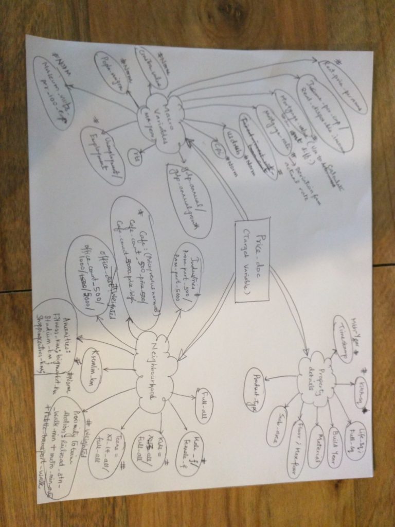
home price analysis mindmap
Hypothesis Qs:
The hypothesis Qs and predictor variables of interest are listed below:
Target Variable: (TV)
“price_doc” is the variable to predict. Henceforth this will be referred to as “TV”.
Predictor variables:
These are the variables that affect the target variable, although we do not know which one is more significant over the others, or indeed if two or more variables interact together to make a bigger impact.
For the Sberbank set, we have predictor variables from 3 categories:
- Property details,
- Neighborhood characteristics,
- Macroeconomic factors
(Note, all the predictors in the mindmap, marked with a # indicate derived or calculated variables).
Property details:
- Timestamp –
- We will use both the timestamp (d/m/y) as well as extract the month-year values to assess relationship with TV.
- We will also check if any of the homes have multiple timestamps, which means the house passed through multiple owners. If yes, does this correlate with a specific sub_area?
- Single family and bigger homes also have patios, yards, lofts, etc which creates a difference between living area and full home area. So we take a ratio between life_sq and full_sq and check if a home with bigger ratio plus larger full_sq gets better price.
- Kitch_sq – Do homes with larger kitchens command better price? So, we will take a ratio of kitch_sq / life_sq and check impact on house price.
- Sub_area – does this affect price?
- Build_year –
- Logically newer homes should have better price.
- Also check if there is interaction with full_sq i.e larger, newer homes gets better price?
- Check inter-relationship with sub_area.
- Material – how does this affect TV?
- Floor/max_floor –
- create this ratio and check affected price. Note, we need to identify how single-family homes are identified, since they would have to be excluded as a separate subset.
- Does a higher floor increase price? In specific sub_area? For example, certain top floor apartments in Chicago and NYC command better price since tenants get an amazing view of the skyline, and there is limited real estate in such areas.
- Product_type – Investment or ownership. Check if investment properties have better price.
Neighborhood details:
- Full_all – Total population in the area. Denser population should correlate with higher sale price.
- Male_f / female_f – Derived variable. If the ratio is skewed it may indicate military zones or special communities, which may possibly affect price.
- Kid friendly neighborhood – Calculate ratio of x13_all / full_all , i.e ratio of total population under 13 to overall population. A high ratio indicates a family-friendly neighborhood or residential suburb which may be better for home sale price. Also correlate with sub_area.
- Similar to above, calculate ratio of teens to overall population. Correlate with sub_area.
- Proximity to public transport: Calculate normalized scores for the following:
- Railroad_stn_walk_min,
- Metro_min_avto,
- Public_transport_walk
- Add all to get a weighted score. Lower values should hopefully correlate with higher home prices.
- Entertainment amenities: Easy access to entertainment options should be higher in densely populated areas with higher standards of living, and these areas presumably should command better home values. Hence we check relationship of TV with the following variables:
- Fitness_km,
- Bigmarket_km
- Stadium_km,
- Shoppingcentres_km,
- Proximity to office: TV versus normalized values for :
- Office_count_500,
- Office_count_1000,
- Logically the more number of offices nearby, better price value.
- Similarly, calculate normalized values for number of industries in the vicinity, i.e. prom_part_500 / prom_part_5000. However, here the hypothesis is that houses nearby will have lower sale prices, since industries lead to noise/pollution, and does not make an ideal residential neighborhood. (optional, check if sub_areas with high number of industries, have lower number of standalone homes (single-family/townhomes, etc).
- Ratio of premium cafes to inexpensive ones in the neighborhood i.e café_count_5000_price_high/ café_count_price_500. If the ratio is high, then do the houses in these areas have increased sale price? Also correlate with sub_area.
Macro Variables:
These are overall numbers for the entire country, so they remain fairly constant for a whole year. However, we will merge these variables to the training and test set, to get a more holistic view of the real estate market.
The reasoning is simple, if the overall mortgage rates are excessive (let’s say 35% interest rates) then it is highly unlikely there will be large number of home prices, thus forcing a reduction the overall home sale prices. Similarly, factors like inflation, income per person also affect home prices.
- Ratio of Income_per_Cap and real_disposable_income: ideally the economy is doing better if both numbers are high, thus making it easier for homebuyers to get home loans and consequently pursue the house of their dreams.
- Mortgage_value: We will use a normalized value, to see how much this number changes over the years. If the number is lower, our hypothesis is that more number of people took larger loans, and hence sale prices for the year should be higher.
- Usdrub: how well is the Ruble (Russian currency) faring against the dollar. Higher numbers should indicate better stability and economy and a stronger correlation with TV. (we will ignore the relationship with Euros for now).
- Cpi: normalized value over the years.
- GDP: we take a ratio of gdp_annual_growth/ gdp_annual, since both numbers should be high in a good economy.
- Unemployment ratio: Uemployment/ employment. Hypothesis is to look for an inverse relationship with TV.
- Population_migration: We will try to see the interaction with TV, while taking sub_area into consideration.
- Museum_visits_per_100_cap: Derive values to see if numbers have increased or decreased from the previos year, indicating higher/lower disposable income.
- Construction_value: normalized value.
In the next posts, we will use a) these hypothesis Qs to understand how the target variable is affected by the variables. (b) Apply the variables in different algorithms to calculate TV.
